Solidly Emissions, a Deep Dive

Summary: We believe public expectations are consistent with the SOLID emissions rate gradually decreasing over ~3 years, but the minter code and historical weekly rebases indicate a much faster tail, with the bulk of emissions distributed over the next 2-3 months.

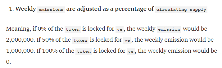
Emissions - public understanding

“The concept is simple, every week SOLID emissions will be distributed starting from 20,000,000 per week decaying at a rate of 2% per week. From week 167, emissions decrease further as the total supply reaches 1 billion SOLID. veSOLID holders decide which liquidity providers receive those emissions.” - Solidex Medium

The public understanding of the Solidly emissions schedule is largely reflective of the statement above. That is, the weekly emissions cap is simply a function of the 2% weekly decay. The weekly emissions cap should in theory look like:

Week 0 - 20M

Week 1 - 98% * 20M = 19.6M

Week 2 - 98% * 19.6M = 19.208M

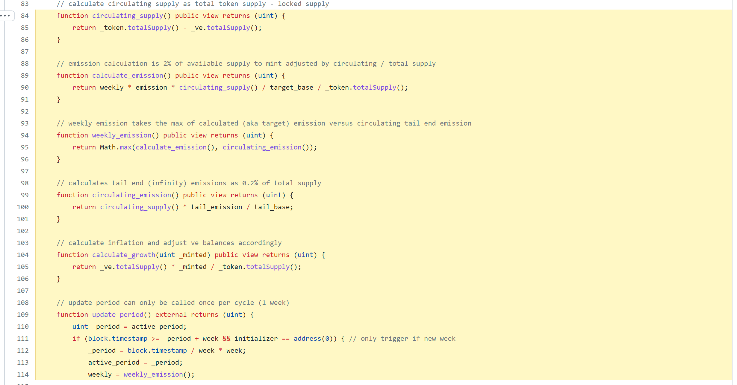
Emissions - our reading of the code

However, a deep dive into the code reveals that this description of emissions schedule is out of line with what the protocol actually does. The BaseV1-minter.sol file contains the logic for the emissions mechanism. The original framing is correct in asserting that the weekly SOLID emissions cap is multiplied by a factor of 0.98, meaning there is a 2% supply cap decay. However, it disregards the presence of another multiplicative factor, the percent of total SOLID that is circulating, which decays the total emissions for that week by the percentage of SOLID that is ve-locked. In particular:

• Line 90 multiplies the supply cap (weekly) by the aforementioned 2% decay (emission/target_base) and the ratio of circulating supply to total supply (circulating_supply()/_token.totalSupply()).
• Line 114 sets the new supply cap for the next week to this week’s emission

Combined, this means that **the supply cap is decreasing from week to week as a function of double decay, in terms of both the well-understood 2% constant decay and the less familiar circulating supply decay.

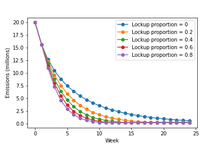
This differs quite substantially from what the original framing indicates for SOLID emissions decay. Exactly how much? The Solidex article posits that by week 167, emissions will tail off as the total SOLID emissions reaches 1 billion. Our analysis reveals that this is far from the case—by our estimate, emissions will taper off by week 15 under the most conservative estimates. Below, we provide plots for the emissions decay with different assumptions about the proportion of SOLID emissions that gets locked up.

It’s worth mentioning that Andre’s original blog post ve(3, 3) explicitly mentions the weighting by the percentage of circulating supply.

How much gets locked?

20 million of ve is effectively perma-locked—therefore, the most conservative estimate of the emissions cap is more accurately modeled by the following function:

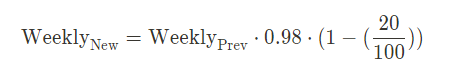
In subsequent weeks, emitted SOLID can be locked (and SOLID that has been locked for its tenure can be unlocked), making it hard to know exactly what the circulating supply proportion will be. But we note that even in the case where no SOLID apart from the original 20 million airdropped ve is locked—the most conservative of estimates, given that this maximizes the circulating supply proportion and therefore the future emissions of SOLID—the total net issuance over the first 167 weeks is 180.10 million SOLID, well below 1 billion. For more perspective on how the reality of SOLID emissions differ starkly from public understanding as set by the Solidex blog post, see Figure 1.

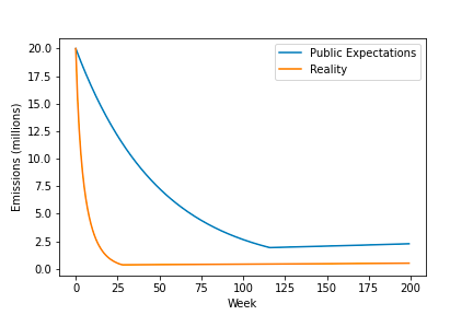
We also emphasize that if more SOLID is locked up beyond the original 20 million, the decay of emissions only accelerates. Figure 2 shows that if the proportion of marginal SOLID emissions that is locked up increases, emissions decline more precipitously.

Testing the hypothesis - observed emissions

As a sanity check, we tested our recreation of how emissions worked against the observed mint amounts for week 1 and 2. If our model was correct, then the first week of emissions after the original 20 million airdrop should have been

as opposed to 19.6 million. We found this matched the actual emissions for week 1.

Then, we took the SOLID lockup rate at the time (which was stable around 25%) and used that to compute our prediction for the weekly emissions for week 2 one day before emissions:

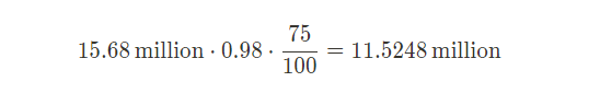
which contrasts greatly to 19.208 million. Indeed, we found that our prediction came fairly close to the actual emissions (10.98 million), with the only discrepancy coming from the exact proportion of SOLID that was locked up (closer to 71.5%). One can track the state of the current weekly emissions cap on FTMScan.

Emissions compared to CRV

CRV is obviously a reasonable comparison point. Many of the design blog posts explicitly referenced CRV. Using the public emissions schedule from https://dao.curve.fi/inflation, we can plot two comparison points: the expected and actual emission schedule for the first 100 weeks (using the most conservative estimate of 0% locked apart from the original 20 MM to NFT holders).

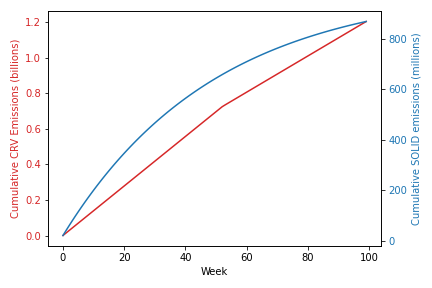
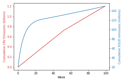
The shape of the above emissions curves is markedly different. Even under the most conservative lock assumptions, a significant majority of the total emissions accrued over 100 weeks is emitted in the first 10 weeks.

Consequences

If the analysis is correct, there are two clear consequences relative to expectations:

1. Lower supply means that each SOLID is a much larger fraction of the fully diluted value
2. The double exponential decay rate leads to a much quicker convergence to the tail emissions value (0.2%).

Is this also how you understand it? Please let us know what we got wrong. Lucas Baker (@sansgravitas), Ben Huan (@HoochieDada), Maher Latif (@maherlatif_), Anirudh Suresh (@anihamde)